Chapter 5
Bayesian Inference
Bayesian inference techniques specify how one should update one’s beliefs upon observing data.
Bayes' Theorem
Suppose that on your most recent visit to the doctor's office, you decide to get tested for a rare disease. If you are unlucky enough to receive a positive result, the logical next question is, "Given the test result, what is the probability that I actually have this disease?" (Medical tests are, after all, not perfectly accurate.) Bayes' Theorem tells us exactly how to compute this probability:
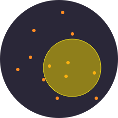
$$P(\text{Disease}|+) = \frac{P(+|\text{Disease})P(\text{Disease})}{P(+)}$$As the equation indicates, the posterior probability of having the disease given that the test was positive depends on the prior probability of the disease \( P(\text{Disease}) \). Think of this as the incidence of the disease in the general population. Set this probability by dragging the bars below.
The posterior probability also depends on the test accuracy: How often does the test correctly report a negative result for a healthy patient, and how often does it report a positive result for someone with the disease? Determine these two distributions below.
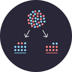
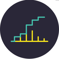
Finally, we need to know the overall probability of a positive result. Use the buttons below to simulate running the test on a representative sample from the population.
| Negative | Positive |
|---|---|
We now have everything we need to determine the posterior probability that you have the disease. The table below gives this probability among others using Bayes' Theorem.
| Negative | Positive | |
|---|---|---|
| Healthy | ||
| Disease |
Likelihood Function
In statistics, the likelihood function has a very precise definition:
$$L(\theta | x) = P(x | \theta)$$The concept of likelihood plays a fundamental role in both Bayesian and frequentist statistics.
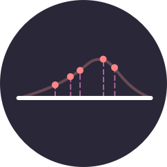
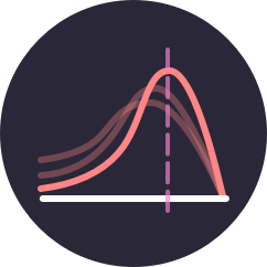
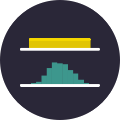
Choose a sample size \(n\) and sample once from your chosen distribution.
Use the purple slider on the right to visualize the likelihood function.
Prior to Posterior
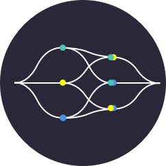
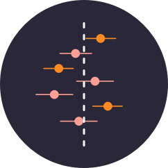
At the core of Bayesian statistics is the idea that prior beliefs should be updated as new data is acquired. Consider a possibly biased coin that comes up heads with probability \(p\). This purple slider determines the value of \(p\) (which would be unknown in practice).
The pink sliders control the shape of the initial \(\text{Beta}(\alpha, \beta)\) prior distribution, the density function of which is also plotted in pink.
As we acquire data in the form of coin tosses, we update the posterior distribution on \(p\), which represents our best guess about the likely values for the bias of the coin. This updated distribution then serves as the prior for future coin tosses.